Plotting Information

Let us plot the data using a time-series scatter plot, and add a trendline.

tidyweather <- tidyweather %>%
  mutate(date = ymd(paste(as.character(Year), month, "1")),
         month = month(date, label=TRUE),
         year = year(date))

ggplot(tidyweather, aes(x=date, y = delta))+
  geom_point()+
  geom_smooth(color="red") +
  theme_bw() +
  labs (
    title = "Weather Anomalies"
  )

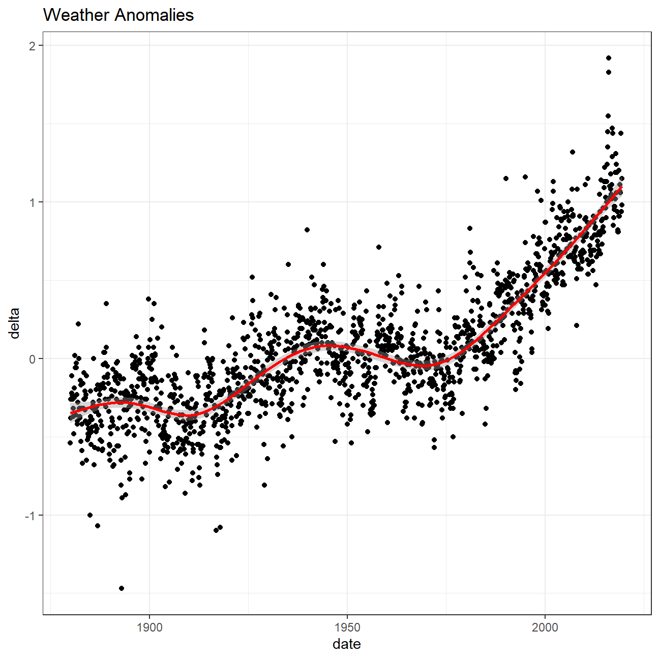
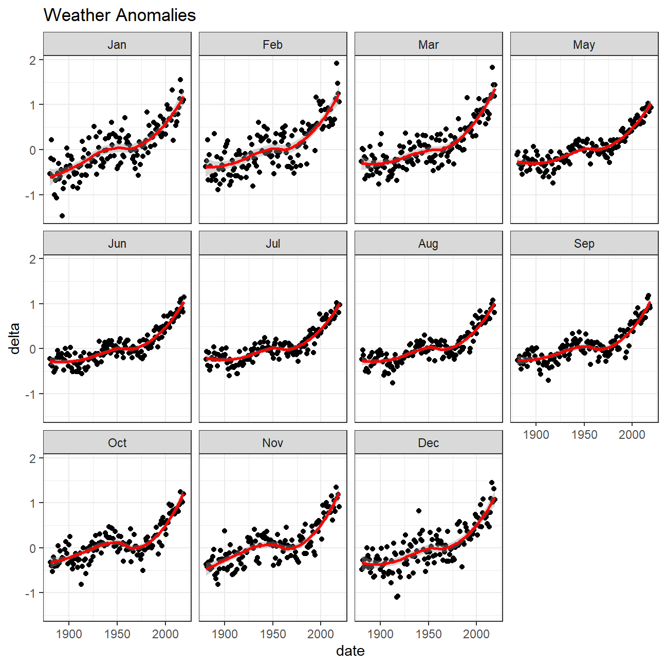
Is the effect of increasing temperature more pronounced in some months? The trend line above shows a significant increase in temperatures. Let’s study it further!

It is sometimes useful to group data into different time periods to study historical data. For example, we often refer to decades such as 1970s, 1980s, 1990s etc. to refer to a period of time. NASA calculates a temperature anomaly, as difference form the base period of 1951-1980. The code below creates a new data frame called comparison that groups data in five time periods: 1881-1920, 1921-1950, 1951-1980, 1981-2010 and 2011-present.

comparison <- tidyweather %>% 
  filter(Year>= 1881) %>%     #remove years prior to 1881
  #create new variable 'interval', and assign values based on criteria below:
  mutate(interval = case_when(
    Year %in% c(1881:1920) ~ "1881-1920",
    Year %in% c(1921:1950) ~ "1921-1950",
    Year %in% c(1951:1980) ~ "1951-1980",
    Year %in% c(1981:2010) ~ "1981-2010",
    TRUE ~ "2011-present"
  ))

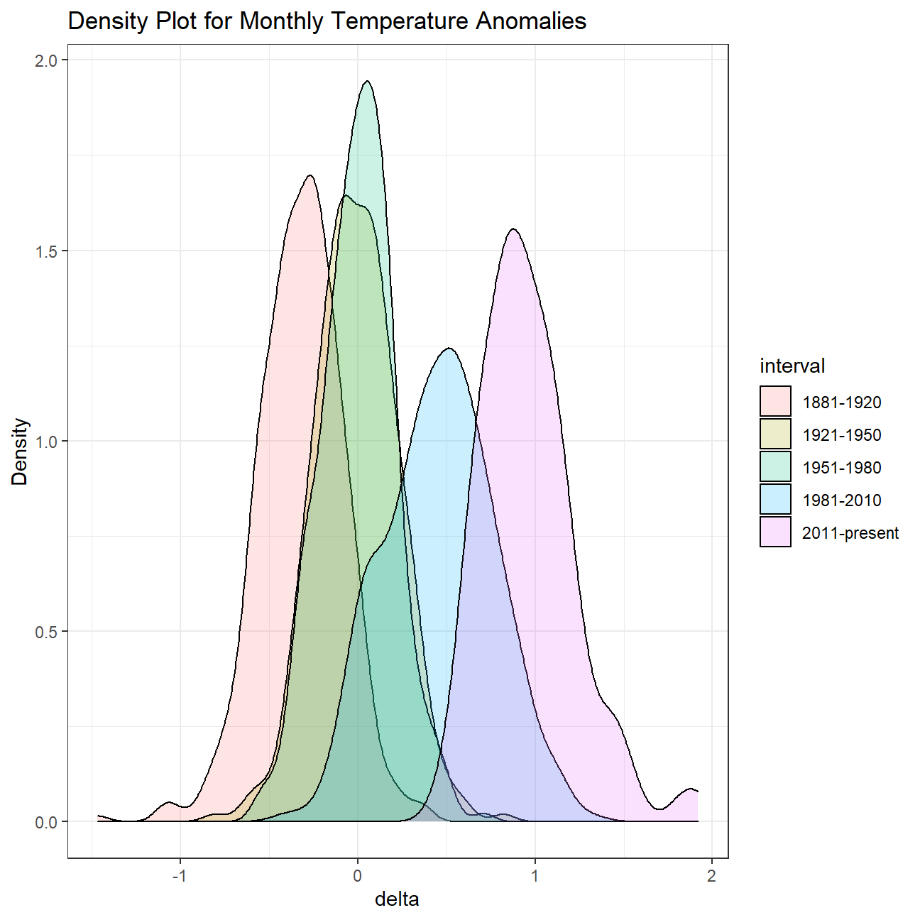
Now that we have the interval variable, we can create a density plot to study the distribution of monthly deviations (delta), grouped by the different time periods we are interested in.

ggplot(comparison, aes(x=delta, fill=interval))+
  geom_density(alpha=0.2) +   #density plot with tranparency set to 20%
  theme_bw() +                #theme
  labs (
    title = "Density Plot for Monthly Temperature Anomalies",
    y     = "Density"         #changing y-axis label to sentence case
  )

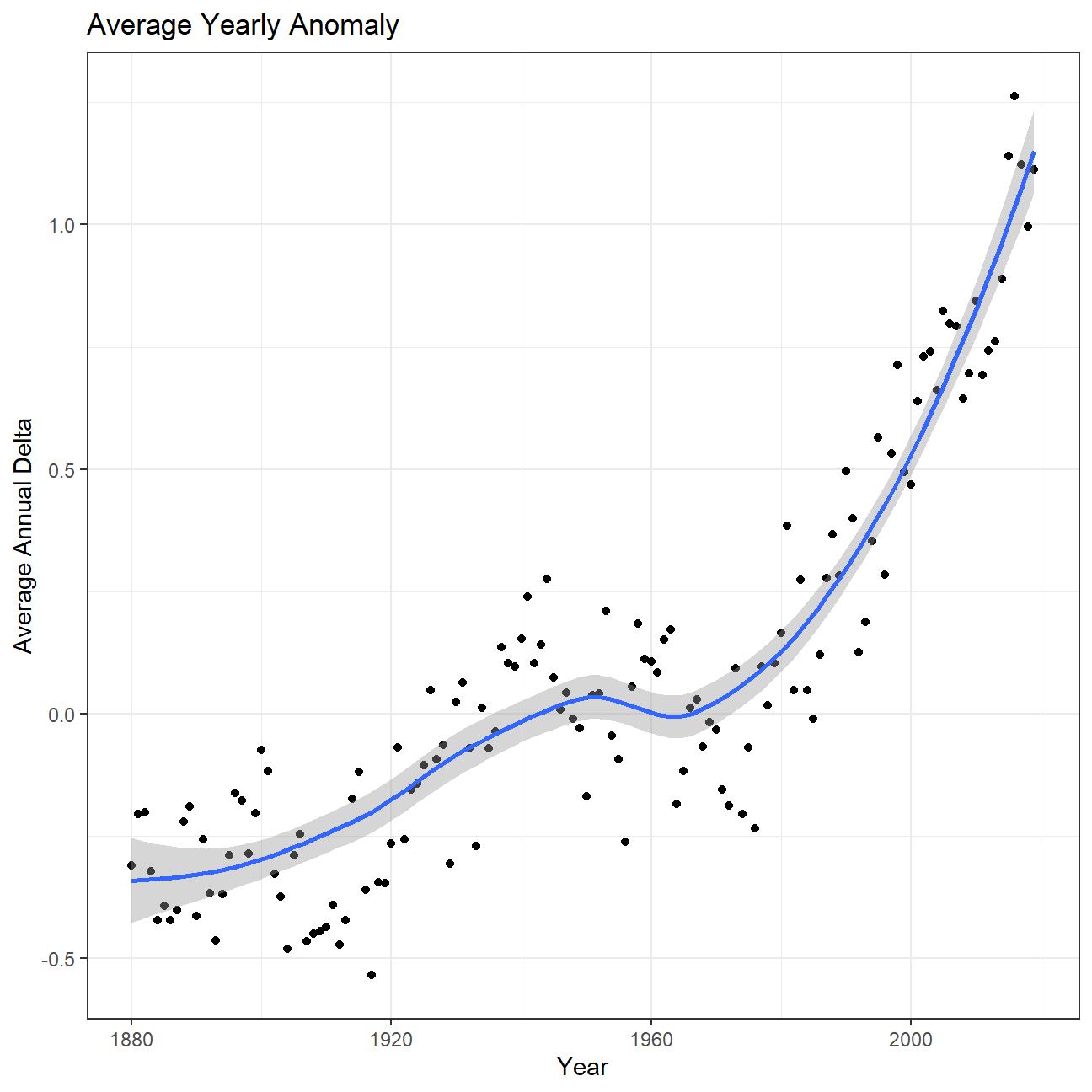
So far, we have been working with monthly anomalies. However, we might be interested in average annual anomalies.

#creating yearly averages
average_annual_anomaly <- tidyweather %>% 
  group_by(Year) %>%   #grouping data by Year
  
  # creating summaries for mean delta 
  # use `na.rm=TRUE` to eliminate NA (not available) values 
  summarise(annual_average_delta = mean(delta, na.rm=TRUE)) 

#plotting the data:
ggplot(average_annual_anomaly, aes(x=Year, y=annual_average_delta))+
  geom_point()+
  
  #Fit the best fit line, using LOESS method
  geom_smooth() +
  
  #change to theme_bw() to have white background + black frame around plot
  theme_bw() +
  labs (
    title = "Average Yearly Anomaly",
    y     = "Average Annual Delta"
  )                         

Confidence Interval for delta

A one-degree global change is significant because it takes a vast amount of heat to warm all the oceans, atmosphere, and land by that much. In the past, a one- to two-degree drop was all it took to plunge the Earth into the Little Ice Age.

We have constructed a confidence interval for the average annual delta since 2011, both using a formula and using a bootstrap simulation with the infer package.

library("infer")

formula_ci <- comparison %>% 

  # choose the interval 2011-present
  # what dplyr verb will you use? 
  filter(interval=="2011-present") %>% 

  # calculate summary statistics for temperature deviation (delta)
  # snippet taken from: https://stackoverflow.com/questions/35953394/calculating-length-of-95-ci-using-dplyr
  summarise(mean = mean(delta, na.rm = TRUE),
            sd = sd(delta, na.rm = TRUE),
            count = n()) %>%
  mutate(se = sd / sqrt(count),
         lower_ci = mean - qt(1 - (0.05 / 2), count - 1) * se,
         upper_ci = mean + qt(1 - (0.05 / 2), count - 1) * se)
  
  # calculate mean, SD, count, SE, lower/upper 95% CI
  # what dplyr verb will you use? 

#print out formula_CI
formula_ci

## # A tibble: 1 x 6
##    mean    sd count     se lower_ci upper_ci
##   <dbl> <dbl> <int>  <dbl>    <dbl>    <dbl>
## 1 0.961 0.267    99 0.0268    0.908     1.01

# use the infer package to construct a 95% CI for delta
formula_ci_infer <- comparison %>% 

  # choose the interval 2011-present
  # what dplyr verb will you use? 
  filter(interval=="2011-present") %>% 

  # calculate summary statistics for temperature deviation (delta)
  group_by(Year) %>% 
  specify(response=delta) %>% 
  generate(reps=100,type="bootstrap") %>% 
  calculate(stat="mean")

#print out formula_CI
formula_ci_infer %>%  get_confidence_interval(level = 0.95,type="percentile")

## # A tibble: 1 x 2
##   lower_ci upper_ci
##      <dbl>    <dbl>
## 1    0.904     1.01

The 95% Confidence Interval values for the average annual temperature delta between years 2011-present is between 0.91C to 1.02C as compared to the base year. This is a worrying result as it represents a significant increase since 2011. Which as mentioned, could lead to major climate changes.