Studying approval margins of Donald Trump
Will he return?
With re-elections in the United States coming close, it is interesting to study the popularity of the current president - Donal Trump. We therefore use detailed data from the website fivethirtyeight.com which provides poll data on Donal Trump.
all polls that track the president’s approval.
In order to fully understand the data, we must first use the glimpse() function before deciding how we must continue our analysis.
# Import approval polls data
#approval_polllist <- read_csv(here::here('data', 'approval_polllist.csv'))

# or directly off fivethirtyeight website
approval_polllist <- read_csv('https://projects.fivethirtyeight.com/trump-approval-data/approval_polllist.csv')

glimpse(approval_polllist)
## Rows: 15,534
## Columns: 22
## $ president <chr> "Donald Trump", "Donald Trump", "Donald Trump",...
## $ subgroup <chr> "All polls", "All polls", "All polls", "All pol...
## $ modeldate <chr> "9/18/2020", "9/18/2020", "9/18/2020", "9/18/20...
## $ startdate <chr> "1/20/2017", "1/20/2017", "1/21/2017", "1/20/20...
## $ enddate <chr> "1/22/2017", "1/22/2017", "1/23/2017", "1/24/20...
## $ pollster <chr> "Morning Consult", "Gallup", "Gallup", "Ipsos",...
## $ grade <chr> "B/C", "B", "B", "B-", "C+", "B+", "B-", "B", "...
## $ samplesize <dbl> 1992, 1500, 1500, 1632, 1500, 1190, 1651, 1500,...
## $ population <chr> "rv", "a", "a", "a", "lv", "rv", "a", "a", "a",...
## $ weight <dbl> 0.680, 0.262, 0.243, 0.153, 0.200, 1.514, 0.142...
## $ influence <dbl> 0, 0, 0, 0, 0, 0, 0, 0, 0, 0, 0, 0, 0, 0, 0, 0,...
## $ approve <dbl> 46.0, 45.0, 45.0, 42.1, 57.0, 36.0, 42.3, 46.0,...
## $ disapprove <dbl> 37.0, 45.0, 46.0, 45.2, 43.0, 44.0, 45.8, 45.0,...
## $ adjusted_approve <dbl> 45.3, 45.8, 45.8, 43.2, 51.6, 37.6, 43.4, 46.8,...
## $ adjusted_disapprove <dbl> 38.2, 43.6, 44.6, 43.8, 44.5, 42.7, 44.4, 43.6,...
## $ multiversions <chr> NA, NA, NA, NA, NA, NA, NA, NA, NA, NA, NA, NA,...
## $ tracking <lgl> NA, TRUE, TRUE, TRUE, TRUE, NA, TRUE, TRUE, TRU...
## $ url <chr> "http://static.politico.com/9b/13/82a3baf542ae9...
## $ poll_id <dbl> 49249, 49253, 49262, 49426, 49266, 49260, 49425...
## $ question_id <dbl> 77261, 77265, 77274, 77599, 77278, 77272, 77598...
## $ createddate <chr> "1/23/2017", "1/23/2017", "1/24/2017", "3/1/201...
## $ timestamp <chr> "15:17:17 18 Sep 2020", "15:17:17 18 Sep 2020",...# Use `lubridate` to fix dates, as they are given as characters.
approval_polllist_dates <- approval_polllist %>%
mutate(enddate = mdy(enddate)) %>%
mutate(week_count = week(enddate)) %>%
mutate(year = year(enddate))
approval_polllist_dates## # A tibble: 15,534 x 24
## president subgroup modeldate startdate enddate pollster grade samplesize
## <chr> <chr> <chr> <chr> <date> <chr> <chr> <dbl>
## 1 Donald T~ All pol~ 9/18/2020 1/20/2017 2017-01-22 Morning~ B/C 1992
## 2 Donald T~ All pol~ 9/18/2020 1/20/2017 2017-01-22 Gallup B 1500
## 3 Donald T~ All pol~ 9/18/2020 1/21/2017 2017-01-23 Gallup B 1500
## 4 Donald T~ All pol~ 9/18/2020 1/20/2017 2017-01-24 Ipsos B- 1632
## 5 Donald T~ All pol~ 9/18/2020 1/22/2017 2017-01-24 Rasmuss~ C+ 1500
## 6 Donald T~ All pol~ 9/18/2020 1/20/2017 2017-01-25 Quinnip~ B+ 1190
## 7 Donald T~ All pol~ 9/18/2020 1/21/2017 2017-01-25 Ipsos B- 1651
## 8 Donald T~ All pol~ 9/18/2020 1/22/2017 2017-01-24 Gallup B 1500
## 9 Donald T~ All pol~ 9/18/2020 1/22/2017 2017-01-26 Ipsos B- 1678
## 10 Donald T~ All pol~ 9/18/2020 1/23/2017 2017-01-24 Public ~ B 1043
## # ... with 15,524 more rows, and 16 more variables: population <chr>,
## # weight <dbl>, influence <dbl>, approve <dbl>, disapprove <dbl>,
## # adjusted_approve <dbl>, adjusted_disapprove <dbl>, multiversions <chr>,
## # tracking <lgl>, url <chr>, poll_id <dbl>, question_id <dbl>,
## # createddate <chr>, timestamp <chr>, week_count <dbl>, year <dbl>Trump’s Average Net Approval Rate
To see how public opinion has evolved over his presidency, We calculated the average net approval rate for each week that Trump has been in office. Doing so helps us study on a more detailed level what factors may have influenced ratings for a certain time-frame. We have filtered the data to ensure only voters are included as their opinions would subsequently be shaping the up-coming presidential elections in 2020.
#Keeping only voters as the subgroup
approval_polllist_dates <-approval_polllist_dates %>% filter(subgroup == "Voters")

#Adding net rate to the data set "approval_polllist_dates"
approval_polllist_dates <- approval_polllist_dates %>% mutate(net_rate = (approve-disapprove)/(approve+disapprove)*100) %>%
  filter(!is.na(net_rate))

#Calculating average net rate on a weekly basis
Weekly_rating <- approval_polllist_dates %>%
  group_by(year,week_count) %>%
  summarise(average_weekly_netrate = mean(net_rate),SD = sd(net_rate), SE = SD/sqrt(length(net_rate)), DF = length(net_rate)-1) %>%
  filter(!is.na(SD))

#Defining confidence intervals
Weekly_rating <- Weekly_rating %>% mutate(CI.upper = average_weekly_netrate+qt(.975,DF)*SE, CI.lower = average_weekly_netrate-qt(.975,DF)*SE)

#Plotting the data
graph_colouring <- c("#FF7733" ,"#81C813", "#2BEEE7", "#ED80FB")

Weekly_rating %>%
  ggplot(aes(x=week_count, y=average_weekly_netrate, color = factor(year))) +
  geom_line() +
  facet_wrap(~year) +
  geom_hline(yintercept =0, color = "orange") +
  scale_x_continuous (limits = c(0,52),breaks=c(0,13,26,39,52),labels = c("0", "13","26","39","52"))+
  geom_point() +
  scale_y_continuous (limits=c(-22,9),breaks=c(-20,-17.5,-15,-12.5,-10,-7.5,-5,-2.5,0,2.5,5,7.5)) +
  geom_ribbon(aes(ymin = CI.lower, ymax = CI.upper, fill = year), alpha=.2) +
  labs(y= "Average Net Approval (%)", x = "Week of the year") +
  ggtitle(label = "Estimating Net Approval (approve - dissaprove) for Donald Trump", subtitle = "Weekly average of all polls") +
  theme(title = element_text(size=8),
        #axis.text.y = element_blank(),
        axis.title = element_text(size=8),
        axis.text = element_text(size=8),
        axis.ticks = element_blank(),
        strip.text = element_text(size=8),
        panel.background  = element_rect(color="black", fill = "white"),
        panel.border = element_blank(),
        strip.background = element_rect(color="black", fill="grey", size=.5),
        panel.grid = element_line(color = "#DCDCDC"),
        legend.position = "none") +
  scale_colour_manual(aesthetics = "custom_color_palette")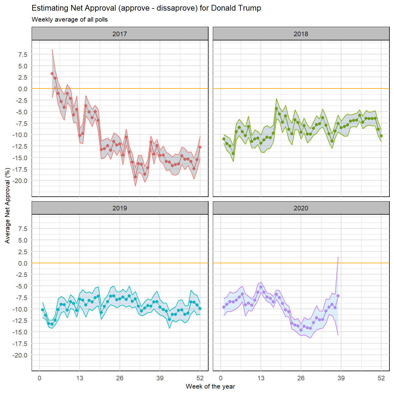
Comparing Trumps Confidence Intervals
What’s going on?
The 95% confidence interval for week 15 (-7.59, -9.09) is relatively narrower than the interval for week 34 (-9.29, -13.16) implying tighter clustering of data near the mean, and lesser dispersion. This translates to a higher proportion of people maintaining their approval rating in week 15, compared to week 34 where the mean approval ratings went further down. One noticeable difference between the two weeks in reference is that the confidence intervals for the approval ratings don’t overlap, and with both the weeks having negative ratings, further downside movement with no overlap to the CI in week 15 doesn’t bode well as re-elections near.
A cause of this variance could be the proximity of re-election date, with more promising candidates (Like Joe Biden) proposing election manifestos contrasting Trump’s policies on response to COVID, racial discrimination and unemployment.
Source: (Burns, Martin and Haberman, 2020)
Citation:Burns, A., Martin, J. and Haberman, M., 2020. In Final Stretch, Biden Defends Lead Against Trump’S Onslaught. [online] New York Times. Available at: https://www.nytimes.com/2020/09/06/us/politics/trump-biden-2020.html [Accessed 8 September 2020].